


Magazine Archive
Home -> Magazines -> Issues -> Articles in this issue -> View
Digital Signal Processing (Part 3) | |
Digital FilteringArticle from Sound On Sound, December 1989 | |
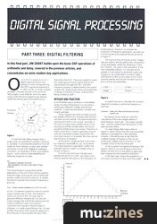
PART 3: In this final part, Jim Grant builds upon the basic DSP operations of arithmetic and delay, covered in the previous articles, and concentrates on some modern day applications.
One of the first applications for a digital signal processor that springs to mind is programming the DSP to generate waveforms. In other words, to create a digital oscillator. The basic process turns out to be fairly simple, as we shall see, but once again using a DSP with all its digital horses packed under the bonnet gives extra performance.

Figure 1.
To start the ball rolling imagine that a single cycle of a waveform is stored in memory, ie. sampled. To animate the waveform the DSP reads out from memory, in turn, each sample and sends it to the DAC (digital-to-analogue convertor). An illustration of this is provided by Figure 1 and could be implemented by the following fragment of code:
DO
INCREMENT MEMORY POINTER
READ MEMORY CONTENTS AND SEND TO DAC
FOREVER
The actual frequency generated will be dependant on the size of the memory used to hold the single cycle and the rate at which the pointer rotates around the memory. A simple formula to calculate the resultant frequency is given by:
Freq = Output sample rate/Memory size for one cycle
So for a 16-element waveform memory and an output sample rate of 1 kHz, the frequency works out to be 62.5Hz. An easy way to generate different frequencies is to vary the output sample rate so that the memory pointer rotates at different rates, but however convenient this may be in terms of ease of software, it is rarely a good thing to do. A major problem that arises from using this approach is the necessity of tracking data recovery filters that follow the DAC. These are needed to reject the image spectra that are generated as the signal passes through the DAC, and their frequency position is determined by the output sample rate. Digital audio filters are problematic to design at the best of times, without them being variable as well!
INTEGER AND FRACTION
A much better way to produce a controllable range of output frequencies is to use what is sometimes called the 'integer and fraction method'. To see how this works, consider two simple examples.
Firstly, suppose we were to rotate around the sample memory at a constant rate but miss out every second sample. The result would be a positive pitch shift of one octave. Secondly, if we were to output every sample twice on our journey around the sample space, the sound would be shifted down one octave. Therefore, it makes sense that in order to generate musical intervals in between simple octave shifts we must skip fractions of a sample. But how can we skip fractions of samples?
At this point it might be best if we invent an imaginary wavetable of, say, 16 locations. The actual waveform type doesn't affect the example, but let's make it a triangle wave as shown in Figure 2.

Figure 2.
To access any particular triangle wave sample and send it to a DAC, we need a 4-bit memory pointer (this gives us the necessary 16 combinations). However, to increase the resolution of frequency generation, we shall use a 16-bit pointer and organise the bits as shown in Figure 3.

Figure 3.
The top four bits are known as the 'integer' and are used to directly address the 16 positions of the wavetable, while the remaining 12 bits, the 'fraction', are used in the calculation of the next wavetable address. To calculate which sample is to be output to generate a particular frequency, we simply add a constant integer and fraction to the current value of the 16-bit memory pointer and use the resultant top four bits to access the wavetable.
A simple formula to calculate the constant required to produce a particular frequency is given by:
Constant = Table size x Required frequency/Output sample rate
The beauty of this method is that the calculation of the new sample address is performed at a fixed rate - the output sample rate - and thus determines the position of the data recovery filters.
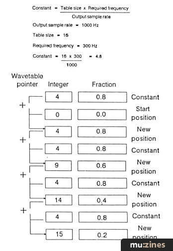
Figure 4.
To make things clear have a look at Figure 4, which shows how the next wavetable address is calculated for a few sampling instants. It should be easy to see that the smallest change of frequency that can be produced is related only to precision, ie. the number of bits of the fractional part.
So far so good, but signal processing is like finance: there is no such thing as a free lunch. Where we lose out is in the ability to generate high frequencies and waveform distortion.
In the best case, where the waveform is a sine wave, we must not skip more than eight samples otherwise we will violate the sampling criterion of needing to generate at least two samples per complete cycle of the waveform, or aliasing will result. For more complex waveforms, which are held in the wavetable, we must limit the skip increment so that the harmonics are not subject to aliasing.
This is where the power of the DSP can step in and arrange for the samples to be generated at a much higher rate than the actual output sample rate, before digitally low pass filtering them and then resampling the result at the correct output rate. This process will ensure the 'fidelity' of the higher harmonics whilst maintaining a fixed and lower output sample rate.
Waveform distortion is the result of two mechanisms, one of which can be cured simply by increasing the accuracy of the samples themselves - in other words, use 16 bits or more. The other headache is the size of the waveform table. Large tables mean that a single cycle of the waveform is accurately represented by many sample values but this increases the number of calculations required to rotate completely around the table. Once again, by using interpolation, the DSP offers a solution.
'Interpolation' is the technique of inventing values between known ones; something we humans do constantly when we look at the time as represented by an analogue watch. The DSP makes use of a reduced waveform table and merely calculates a more accurate sample value from the history of previous values and the future ones.
DIGITAL FILTERING
The field of digital filtering is vast and increasingly popular with the pundits of audio signal processing, despite the enormous problems created when trying to digitally represent highly resonant systems with a limited arithmetic resolution. Fortunately, we can ignore such difficulties and concentrate on the interesting aspects of digital filters.
Many digital filters are merely copies of analogue filters represented in the digital domain, and in general there are two basic types: infinite impulse response (IIR) and finite impulse response (FIR) filters. IIR filters are characterised by the presence of feedback, where the current output sample is calculated (using delay lines) from the history of the input samples and the history of the output samples. Clearly, if the past output samples are involved in the generation of a new output sample, then a situation can arise where the output increases without respite. Too much feedback can occur, which is not the sole prerogative of the digital domain, of course. On the other hand, FIR filters calculate their new output samples solely by considering the input samples, so feedback can never occur.
Constant = (Table size x Required frequency) / Output sample rate
Output sample rate = 1000 Hz
Table size = 16
Required frequency = 300 Hz
Constant = (16 x 300)/1000 = 4.8
As an example ot a powerful and commonly used digital filter, we shall concentrate on the FIR type. The exact meaning of the term 'FIR' will help to explain the operation of this type of filter...
To design a filter, we usually specify its performance in the frequency domain: cut-off frequency, roll-off slope, Q or resonance etc. This is fine, and a good way to proceed, because we often view the result of a filter's action in the frequency domain, ie. which frequencies are passed or rejected. However, the action of any system - be it filters, amplifiers or anything else - can also be viewed in the time domain, instead of the usual frequency domain.
If we pass a signal through a filter, then its frequency content may well be altered with the result that the filter, in effect, outputs a 'different' waveform. We can describe the action of the filter in terms of either the frequency content changes to the signal or the waveform changes. Thus we have a frequency domain description or a time domain description (nobody said this would be easy, only interesting!).
As it turns out, a particularly useful signal with which to obtain the description of a system in the time domain is one called the 'unit impulse'. It has the property that all signals can ultimately be composed of unit impulses, and if we know the time response of a filter from a unit impulse then we know its response to all other signals. This can be extended to the principle that if we define the action of a filter by its time response, then we automatically determine its frequency response also.
With this knowledge, we can now design a filter by specifying its behaviour in the frequency domain (as usual) but digitally model its performance to a unit impulse (and therefore all other signals as well). We effectively end up with the same filter only implemented a different way.

Figure 5.
A typical FIR filter is shown in Figure 5. The filter consists of a chain of delay elements, each of which passes its sample content to the element on its right at the sample rate. This is a common arrangement in digital electronics, and is often called a 'shift register'. At each sampling instant, the output sample is calculated by multiplying the sample contained in each delay element (S0 to S9) by the number held in the box below (M0 to M9), and then adding all the results together. This amounts to a lot of arithmetic, and really requires the power of a DSP.
It is not difficult to see what the system does to generate the output samples but we still have to make the connection with unit impulses. The trick is this: the numbers (M0 to M9) which multiply the samples held in the delay line are values of the impulse response at different (later) instants in time. When each sample traverses along the delay line the output will consist, in part, of the impulse response due to that individual sample. Since the delay line will hold many samples at once, the complete output is the sum of all the delayed impulse responses of each sample as they move along the delay line. The curve above the delay line (Figure 5) is drawn to show the impulse response generated by an individual sample, with the corresponding value held in the multiplier boxes.
CONVOLUTION
Although we have described the operation of a FIR filter, the general principle of summing impulse responses is called convolution. If we take things just a step further, we can see that convolving the input signal with the impulse response is the same as multiplying the frequency content of the signal with the frequency response of the filter. Stated simply: convolution in the time domain is equivalent to multiplication in the frequency domain, and this is generally known as 'filtering'.
In concluding this brief series, we have come a long way from simple arithmetic to produce mixers and gain blocks, to convolution and FIR filters. In case you think that this all seems a bit esoteric and complicated, have a read of Paul Wiffen's 'Tokyo Music & Sound Expo' report (p97, SOS November 1989) or page 10 of this issue; there you will find descriptions of the new SY77 wonder synth from Yamaha, which employs a method of synthesis called 'RCM' - Real-time Convolution and Modulation. Is this just another name for filtering? Time will tell...
Series - "Digital Signal Processing"
This is the last part in this series. The first article in this series is:

Digital Signal Processing
(SOS Oct 89)
All parts in this series:
More with this topic
 Aural Examination - Aural Exciters |
 Routing Enquiries |
 To Phase or to Flange - Or To Each His Own |
 Reverberation |
 Dateslate |
 Build a Modular Vocoder |
 A Chorus Line-Up - Which Chorus? |
 Outboard |
 Hi-Fi Graphics |
 Digital Effects - A Guide to Digital Reverbs, Delays and Multi-Effects Units |
How To Do Tricks With Time |
 Signal Processing With Sequencers |
Browse by Topic:
Effects Processing
Publisher: Sound On Sound - SOS Publications Ltd.
The contents of this magazine are re-published here with the kind permission of SOS Publications Ltd.
The current copyright owner/s of this content may differ from the originally published copyright notice.
More details on copyright ownership...

Sound On Sound - Dec 1989
Donated & scanned by: Mike Gorman
Feature by Jim Grant
Previous article in this issue:
Next article in this issue:
Help Support The Things You Love
mu:zines is the result of thousands of hours of effort, and will require many thousands more going forward to reach our goals of getting all this content online.
If you value this resource, you can support this project - it really helps!
Donations for May 2026
Issues donated this month: 0
New issues that have been donated or scanned for us this month.
Funds donated this month: £0.00
All donations and support are gratefully appreciated - thank you.
Magazines Needed - Can You Help?
Do you have any of these magazine issues?
If so, and you can donate, lend or scan them to help complete our archive, please get in touch via the Contribute page - thanks!